Nondestructive measurements were made on whole sections of core using the multisensor track (MST). This incorporated the Gamma Ray Attenuation Porosity Evaluator (GRAPE), P-wave logger (PWL), and magnetic susceptibility sensors. Thermal conductivities were measured for sediments and basement rocks using the needle probe method. When the sediment was soft enough, compressional wave velocities, undrained shear strengths, and electrical resistivities were measured on the working half of the core. In addition, discrete samples were taken throughout the cores for determining index properties and compressional wave velocities.
The MST incorporates the GRAPE, PWL, and magnetic susceptibility sensors. A natural gamma-ray sensor was added to the MST at the beginning of Leg 149, which was used only on selected cores for testing the instrument. Individual unsplit core sections were placed horizontally on the MST, which moves the section past the four sensors.
The GRAPE measures bulk density at 1 cm intervals (minimum) by comparing the attenuation of gamma rays through the cores with attenuation through aluminum and water standards (Boyce, 1976). The GRAPE data are most reliable in APC and fullsized XCB and RCB cores and offer the potential of direct correlation with downhole bulk density logs. For the preliminary on-board processing, only every 20th measurement was used. Corrections were made for variations in core diameter, pore water composition, and mineralogy, following Evans and Cotterell (1970), Boyce (1976), and Lloyd and Moran (unpubl. data). For very disturbed cores, the GRAPE acquisition was turned off.
The PWL transmits a 500-kHz compressional-wave pulse through the core at a repetition rate of 1 kHz. The transmitting and receiving transducers are aligned perpendicular to the long axis of the core. A pair of displacement transducers monitors the separation between the compressional wave transducers; variations in the outside diameter of the liner therefore do not degrade the accuracy of the velocities. Measurements are taken at 3-cm intervals. Generally, only the APC and fullsized XCB and RCB cores were measured. The quality of the data was assessed by examining the arrival time and amplitude of the received pulse. Data having anomalously large traveltimes or low amplitudes were discarded.
Magnetic susceptibility was measured on all sections at intervals of 3 to 5 cm using the 1.0 range on the Bartington Instruments magnetic susceptibility meter (model MS2) with an 8-cm-diameter loop. The magnetic susceptibility provides another measure to assist cross-hole correlations and can help to detect fine variations in magnetic intensity associated with magnetic reversals. The quality of these results degrades in XCB and RCB sections where the core liner is not completely filled and/or the core is disturbed. However, the general downhole trends may still be used for stratigraphic correlation.
Whole-round core sections were allowed to adjust to room temperature for at least 4 hr before measuring thermal conductivities. The needle probe method was used in full-space configuration for soft sediments (Von Herzen and Maxwell, 1959), and in half-space mode for lithified sediment and hard rock samples (Vacquier, 1985). Thermal conductivities were typically measured in alternate sections. During transit to the first site and at irregular intervals during the cruise, the needle probes were calibrated vs. known standards (red rubber, black rubber, and macor), providing for five measurements in each standard per needle. A least-squares linear regression of known thermal conductivity and measured conductivity was performed for each needle to provide the corrections used for data reduction. Data are reported in units of (W/m·K), with an uncertainty of 5% to 10%, estimated from the regression line.
Needle probes, containing a heater wire and a calibrated thermistor, were inserted into the sediment through small holes drilled into the core liners before the sections were split. The probes were positioned where the sample appeared to show uniform properties. Data were acquired using a Thermcon-85 unit interfaced to an IBM-PC compatible microcomputer. This system allowed up to five probes to be connected and operated simultaneously. For quality control, one probe was used with a standard of known conductivity during each run.
At the beginning of each measurement, temperatures in the samples were monitored without applying current to the heating element to verify that temperature drift was less than 0.04°C/min. The heater then was turned on and the temperature rise in the probes was recorded. After heating for about 60 s, the needle probe response behaves nearly as a line source with constant heat generation per unit length. Temperatures recorded between 60 and 240 s were fit to the following equation using the least-squares method (Von Herzen and Maxwell, 1959):
![]()
where k is the apparent thermal conductivity (W/m·K), T is temperature (°C), t is time (s), and q is the heat input per unit length of wire per unit time. The term L(t) corrects for a linear change in temperature with time, described by the following equation:
where A represents the rate of temperature change, and Te is the equilibrium temperature. L(t) therefore corrects for the background temperature drift, systematic instrumental errors, probe response, and sample geometry. The best fit to the data determines the unknown terms k and A.
Half-space measurements were performed on selected lithified sediments and crystalline rock samples after the cores were split and the faces of the split cores were polished. The needle probe rested between the polished surface and a grooved epoxy block having relatively low conductivity (Sass et al., 1984; Vacquier, 1985). Half-space measurements were conducted in a water bath to keep the samples saturated, to improve the thermal contact between the needle and the sample, and to reduce thermal drift. EG&G thermal joint compound was used to improve the thermal contact. Data collection and reduction procedures for half-space tests are similar to those for full-space tests, except for a multiplicative constant in Equation 3 that accounts for the different experimental geometry.
Index properties, including bulk density, grain density, water content, and porosity, were calculated from measurements of wet and dry sample masses and wet volumes. On samples of approximately 10 cm3 dry sample volumes, which can be determined indirectly from the raw measurements listed above, also were measured directly, allowing one to check the calculations. In addition, bulk density was measured on unsplit cores using the GRAPE, as discussed above.
Sample mass was determined to a precision of ±0.01 g using a Scitech electronic balance. The sample mass was counterbalanced by a known mass such that the mass differentials generally were less than 1 g. Sample volumes were determined using a Quantachrome Penta-Pycnometer, a helium-displacement pycnometer with a nominal precision of ±0.02 cm3, but a lower apparent experimental precision. Sample volumes were measured at least twice, and the mean of the readings was taken to be the volume. A reference volume was run with each group of samples, and rotated among the cells to check for systematic error. This exercise demonstrated that the measured volumes had a precision of about 0.03 cm3. The pycnometer volumes were re-calibrated frequently during use for both small and large sample holders. The sample beakers used for discrete determinations of index properties were calibrated carefully prior to the cruise.
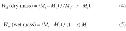
There are two definitions for pore-water content: (1) Wd, pore-water mass divided by the mass of solids Ms, and (2) Ww, pore-water mass divided by total mass Mt. When determining water content, the methods of the American Society for Testing and Materials were followed (ASTM, designation [D] 2216; ASTM, 1989). The total (Mt) and dry (Md) masses were measured using the electronic balance. The difference (Mt-Md), after correction for salt by assuming a pore-water salinity (r) of 0.035, following the discussion by Boyce (1976), was taken as the pore-fluid mass. The equations for the two water-content calculations are as follows:
Bulk density (ρ) is the density of the total sample including the pore fluid (i.e., ρ = Mt/Vt, where Vt is the total sample volume [cm3] measured with the helium pycnometer).
Grain density, ρg is determined from the dry mass (Scitec balance) and dry volume (pycnometer) measurements. In this case, both mass and volume must be corrected for salinity, leading to the following equation:
is the density of salt (2.257 g/cm3).
![]()
where Vd is the dry volume (cm3) and ρs is the density of salt (2.257 g/cm3). Ms = r · Mw is the mass of salt in the pore fluid, Mw is the mass of the seawater:
![]()
To check these determinations, and to assess the quality of the volumes derived from the helium pycnometer, grain density was estimated occasionally using dry volume measurements in powdered samples.
Porosity (η), the ratio of the fully saturated pore-water volume to the total volume, can be determined several ways using the quantities derived above. The following relationship using calculated grain density, ρg, and bulk density ρ was employed:
![]()
where ρg is grain density, ρ is bulk density and ρw is seawater density. To check for internal consistency, porosities also were calculated using the relationship:
![]()
where ρ is bulk density and Wd is water content (dry mass).
Discrete compressional-wave (P-wave) velocity measurements were obtained using two different systems, depending on the degree of lithification of the material. A Digital Sound Velocimeter (DSV) is a digital data acquisition system developed to measure and record compressional wave velocities and attenuation in soft sediments. The velocity calculation is based on the traveltime of an acoustic impulse between two piezoelectric transducers that are inserted directly into the split core. The transducers emit a 2-s pulse having a repetition rate of 60 Hz. Gains from 0 to 42 dB can be applied to the received signal. The transmitted and received signals are displayed by a Nicolet 320 digital oscilloscope and transferred to a microcomputer for processing. The DSV software sums the waveforms from 3 to 10 successive digital records and displays the resulting waveform on the oscilloscope. Traveltime is estimated by visual identification of the first break on the stacked waveform and is corrected for the total delay caused by the transducers and other velocimeter hardware. Velocity is determined from the corrected traveltime and the measured distance (by caliper) between the transducers. The traveltime correction was determined by measuring the velocity of a distilled water sample and comparing the result to the standard water velocity (Wilson, 1960).
The Hamilton Frame Velocimeter (Hamilton, 1971) was used to measure compressional-wave velocities for well-indurated sediments, lithified sediments, and crystalline rocks. Velocity was determined using an impulsive signal having a frequency of 500 kHz. Cubes were trimmed from the sediment samples using a knife, with faces oriented parallel to the axis and split surface of the core. Velocity was measured in three mutually perpendicular directions, V (along the core axis), Hx (perpendicular to core axis and parallel to core face), and Hy (perpendicular to core face). The magnitude of acoustic anisotropy was estimated according to the relationship:
![]()
where Vmax and Vmin are the maximum and minimum velocities (among V, Hx, and Hy). In crystalline rocks minicore samples (2.54-cm diameter) were drilled perpendicular to the axis and face of the core. The ends of the minicores were trimmed parallel with a rock saw, and velocity (Hy) was measured along the axis of the minicore. Whenever possible, velocity measurements were made adjacent to paleomagnetic measurements, to allow the possibility of orientating the samples to geographic coordinates.
The dimensions of samples measured in the Hamilton Frame were determined with a digital linear caliper. Traveltime was estimated by visual identification of the first break of the stacked waveform, as described for the DSV measurements. Traveltime was corrected for the total delays caused by the transducers and velocimeter hardware. This was estimated by a linear regression of traveltime vs. distance for a series of aluminum and lucite standards. Velocities were calculated from the corrected traveltimes and measured sample dimensions. Velocity data are reported here in raw form; however, corrections to in-situ temperature and pressure also can be made using the relationships in Wyllie et al. (1956).
Resistivity was measured during Leg 149 using a four-probe configuration (Wenner spread) having two current and two potential electrodes. The electrodes, separated along the axis of the core, were pushed approximately 2 mm into and normal to the split core surface. The resistance of the saturated sediment was derived from the potential difference and instrument current using Ohm's law.
The resistivity data for the sediments are presented in terms of the formation factor (FF), which is the ratio of the resistivity of the saturated sediment to the resistivity of the pore fluid. The resistivity of the pore fluid was assumed to be the same as that of seawater (Boyce, 1980). The FF was calculated by dividing the resistance of the sample by the resistance of the seawater at room temperature, measured with the same apparatus. For consolidated sediments and hard rocks, electrical resistivity was measured in drilled minicores using an electrical resistivity cell.
The undrained shear strength (Su) of the sediment was determined using a Wyckham-Farrance motorized miniature vane shear device following the procedures of Boyce (1977). The vane rotation rate was set to 90°/min. Measurements were performed only in the fine-grained units having soft consistencies. The vane used for all measurements has a blade height of 1.27 cm and a diameter of 1.27 cm.
The instrument measures and records the torque and strain at the vane shaft using a torque transducer and potentiometer, respectively. The shear strength reported is the peak strength determined from the torque vs. strain plot. The residual strength is given by the steady-state strength of the material following failure (Pyle, 1984). It is assumed during this test that a cylinder of sediment shears uniformly about the axis of the vane in an undrained condition, and cohesion is the principal contributor to shear strength. However, progressive cracking within the sediment, pore pressure drainage, or local inhomogeneities can degrade the quality of the measurements.
![]()