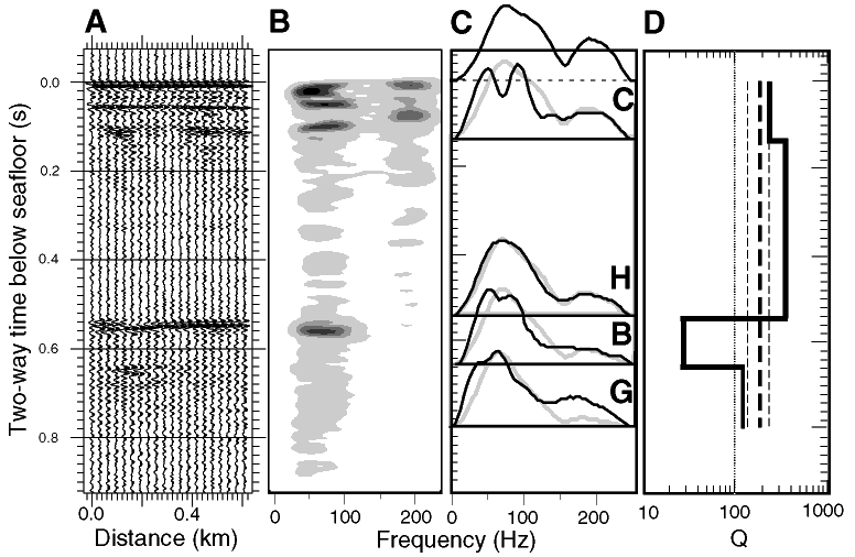
Figure 4. To invert for Q, a suite of 20 traces (A) is transformed into time vs. frequency (B; the darker shades represent higher amplitudes). (C) The spectra from around selected layers (dark lines) are modeled using an automated iterative forward modeling scheme (simulated annealing), resulting in a set of synthetic spectra (gray curves), and (D) the corresponding Q profile of the sediments (solid line). Inverting the same spectra for a constant Q yields the bold, dashed curve, with uncertainties shown as fine, dashed lines.

![]()