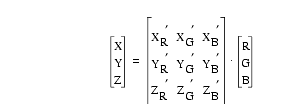
 , (1)
, (1)
The imaging system that was used during Leg 167 consisted of a SONY DXC-750MD NTSC camera with three charge-coupled device (CCD) arrays of 768 × 493 cells and a Fujinon TV.Z 4 × 7.5 lens. The camera registers the three channels, red (centered at 700 nm), green (546 nm), and blue (436 nm), simultaneously, which reduces the possibility that shipboard vibration will affect the quality of the image. For lighting, two 200-watt, daylight-balanced Hydrargyrum Medium Arc Iodide (HMI) lamps were used, which have an initial color temperature of 5600°K. The manufacturer stated that the color temperature of the lamps would decrease at a rate of 1°K/hr. In practice, however, the color temperature trend turned out to be less predictable.
Cores were imaged in steps of 20 cm, with each image originally having an overlap with surrounding images, covering around 25 cm of sediment in a 24-bit image of 1008 pixels along the core axis by 486 pixels across the width of the core. To reduce storage requirements as much as possible, all images were trimmed automatically, reducing the overlap to 0.3 cm. The effective resolution along the stratigraphic axis translates into ~40 measurements (pixels) per centimeter of sediment (0.25 mm).
With each segment of sediment, a ruler was photographed with a black and white bar code that would allow automated recognition of the exact interval within a 1.5-m section. Each image also contains a color reference card with red, green, blue, gray and white chips, for which the color values in the XYZ tristimulus color space have been determined for ODP. These reference chips are used for calibration of absolute color values of the sediments.
Time series are extracted from the images by extracting RGB values along a line through the image, converting the values to CIE L*a*b*, correcting each interval for inhomogeneities in the light distribution of the bulbs, and stacking all segments to a continuous time series. This process was fully automated during the cruise, to produce a preliminary time series while keeping up with the core flow. The reprocessing of the images that will be described here is only semiautomated. The various steps in the processing are done on all images in one run, but after each step, results are written to disk and checked for consistency. For each step, several relevant variables that summarize the results were plotted to be able to detect outliers that were due to incorrect handling of the data in a specific image. For example, correct recognition of the bar code, used to produce a depth scale, can be checked by plotting the calculated resolution for all images, as errors will result in aberrant values in pixels per centimeter of sediment. The actual order in which the various processing steps are done (e.g., color calibration, correction for inhomogeneous light distribution of the illuminant, filtering out of cracks and voids) is in itself not crucial; the order used here is mainly chosen for convenience.
In each image, a line scan of one pixel wide was collected at a fixed position in the image, which corresponds to approximately the center of the core surface. With the line scan, a line of pixels was collected from within the bar code, and the average RGB values were calculated for a 40 by 20 pixels large area from each of the red, green, blue, and gray chips on the color card. With these raw data as the basic input, the following steps were done to obtain the final filtered color time series.
As a first step in the processing, measured RGB values in the line scan are converted to CIE L*a*b*. L* describes lightness; its values can range between 0 (black) to 100 (white). The other two variables describe the actual color, with a* representing green (negative values) or red (positive) and b* representing blue (negative) or yellow (positive values). CIE L*a*b* has as an advantage over other color systems because the three variables are the most easy to interpret in color as registered by the human observer. Translation into the L*a*b* system is done via an intermediate step, by translating RGB values into CIE XYZ (tristimulus) values. This intermediate step is crucial in obtaining calibrated color results that are reproducible independent of which camera system, light source, or calibration setting is used. The standard conversion from RGB to XYZ values, which was used shipboard, uses the following equation (Rogers, 1985):
 , (1)
, (1)
where
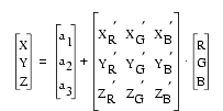
However, for computational purposes, the terms (XR · CR), (YR · CR), (ZR · CR), and so on are taken together as a single unknown constant each, giving
 . (2)
. (2)
Equation 2 can be solved by inserting measured RGB values and known XYZ values for each of the red, green, and blue chips that were photographed with each segment of core. Writing out the three matrix multiplications and rearranging the equations yields three sets of three linear equations with three variables each.
This standard conversion implies that the lines calculated for X, Y, and Z intersect the origin of the axes (i.e., that pure black has values equal to, or very close to (0,0,0) in both the XYZ and RGB vector space). In practice, Equation 2 could not adequately estimate color values to give the same absolute values before and after a recalibration of the camera, which was done to correct for drift in the green channel. Therefore, Equation 2 was modified to allow for the presence of an offset from the origin, to take into account that the actual values produced by the camera for black and white are dependent on the setting
 . (3)
. (3)
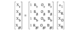
In this case, information about four colors is needed to solve the constants (i.e. the red, green, blue, and gray chips). Writing out the matrix multiplication and rearranging the sets of linear equations yields the following for the X-values of the four color chips used:
 . (4)
. (4)
Here, Rr, Gr, and Br, and Xr, Yr, and Zr are the measured video camera channels and the known XYZ values respectively for the red chip; subscripts g = green, b = blue, and gr = gray apply to the other three color chips used. This set of four linear equations with the four required constants as variables can be solved with standard methods; Y´ and Z´ constants are solved in an equivalent manner.
Equation 4 and its equivalents for Y´ and Z´ are solved for each image individually. Results show that the introduction of a vector of constants produces a better approximation of absolute color values than the standard three by three matrix conversion. Typically, values for the constants a1, a2, and a3 are found to range between 1.5 and 4.5, demonstrating that an offset from the origin of the X, Y, and Z axes is indeed present. The result of the four-variable approach, after further conversion to L*a*b* values, produces similar values for parallel holes imaged before and after recalibration of the video camera (Fig. 1B). The four-variable matrix solution uses all the color information in the reference color card that was scanned with each image for this study (the white chip in the card is usually out of gamut). However, a reference card with more than four color chips would allow the constants to be solved for various combinations of four colors, thereby allowing statistical averages to be estimated.
The XYZ values estimated for the data in the line scan are then further converted to CIE L*a*b* values using the following equations (from Billmeyer and Saltzman, [1981]):
 , (7)
, (7)
with f(Y/Yn)
= (Y/Yn)1/3
for Y/Yn
> 0.008856 and f(Y/Yn)
= 7.787(Y/Yn)
+ 16/116 for Y/Yn
![]() 0.008856; f(X/Xn)
and f(Z/Zn)
are defined similarly. Xn,
Yn, and Zn
are the tristimulus values of a reference white. For this study, the known XYZ
values of the white color chip are used as reference values.
0.008856; f(X/Xn)
and f(Z/Zn)
are defined similarly. Xn,
Yn, and Zn
are the tristimulus values of a reference white. For this study, the known XYZ
values of the white color chip are used as reference values.
The conversion to L*a*b* is done as the first step, to facilitate detection of voids and cracks in the sediments, which in this color system can be easily recognized in the single variable L*, whereas all three variables are needed in other systems. Cracks in the sediments result in pixels that are darker than the surrounding sediment (have lower L* values) or, if voids are filled with foam, as much lighter pixels. Considering all values in one segment as a statistical distribution (or histogram), such voids and cracks should show up as outliers. For this study, extremes on either side of the distribution were removed, using as truncation limits (determined by trial and error) the first one-unit wide frequency class on either side with more then 10 measurements. The resulting truncation was checked by plotting the resulting maximum and minimum L* values for consecutive images. Segments with aberrant values were then inspected manually and adjusted if required. All values that were finally identified as outliers were then set to missing data. This includes voids and cracks, as well scratches in the core surface that produced dark shadows or very strong reflections. To compile an optimal time series, gas voids, which artificially add to the thickness, should actually be subtracted from the composite depth scale. However, the present color data set retains the curated composite depth scale, to allow correlation with other data.
The images have to be corrected for the effect of a nonuniform distribution of the light source. The actual light distribution produced by the lamps across the imaged area can be estimated by measuring the departure from average in an image of a uniform gray card. However, this estimated light distribution, which was used shipboard to correct for light effects, is in practice not suitable to remove all artifacts from the sediment color time series. The actual departure from a flat line across an image depends largely on how reflective the imaged material is. The effective light distribution in sediment, which is wet, especially in the top cores, is more steeply curved than the distribution across the dull gray cards that were scanned for reference. The ruler in the image has a light curve that is again more steeply curved than the sediment (Fig. 2). The video system on board was not polarized. However, reflections produced by wet sediment can be reduced by polarization, but cannot be suppressed completely. For example, the shore-based ODP Leaf-digital imaging system, which is polarized, still produces sediment light curves that are steeper than those across a dull surface.
The result is that light correction can only use the sediment itself to estimate the departure from a flat line across an image that a homogeneously colored surface gives. As wetness of the sediment, and thus reflectivity, will vary from section to section, a light correction curve should be estimated for each image individually. One method would be to use the overlap between adjoining images. Although the steepness of the measured light curve varies, the basic shape remains constant. Using an overlap of several centimeters, the correction could be done by flattening the measured curves progressively until the best fit between pairs of overlapping images is obtained. This approach could not be tested as a method because the present data set does not have enough overlap between images to produce reliable results.
Light correction here was finally done by fitting polynomial least-square regression lines to each of L*, a*, and b* in each image, using pixel position within the line scan as the independent variable in the regression. However, the best-fit curve in a given individual segment will incorporate real variation in sediment color as well as the effects of the nonuniform distribution of the light source. By taking the average curve for a large set of images any systematic variation in real color at a decimeter scale, which will affect curves in individual images, is filtered out as it does not occur systematically in the same position in all images. In this case, we estimated one average light correction curve for each site separately. The departure from the mean of the values in the correction curve was then subtracted from the values in each line scan to correct for light distribution. The approach used here, while reducing the effects of the light source, cannot completely remove all artifacts, however, because a single average curve cannot account for steeper or flatter distributions in individual images. Indeed, some 20-cm cyclicity remains present in all sections as an artifact of light distribution, but in most sites the amplitude is much lower than that of the real color variation. However, for Site 1019, which has sediments that show only subtle variation in color, using the average regression curve for all images produced results in which a considerable amount of the total variation in color could be attributed to light distribution artifacts. Therefore, for Site 1019, several regression curves were calculated (i.e., for the top two cores in all holes together, and than for all remaining cores in each hole separately).
Further distortion in the color-data color is produced by the end-of-section markers, which were included as an aid in the automated processing. The markers, which lie on top of the split core liner, consist of white foam, edged with red (or blue) tape. Apparently, light reflects from this tape onto the sediment in the immediately adjoining part of the core surface. At least in practice, the 10 cm or so of sediment close to the end-of-section marker is found to give values in all three color variables that are consistently different from values in the rest of the section. The offset is only a few units, but it is large enough to be noticeable unless the real color variation has a high amplitude. To avoid potential artifacts, the deepest 10 cm in all sections was deleted from the final data set presented here.
The high resolution of 40 measurements per centimeter that is obtained from the images after the processing described above is not required to describe the usually decimeter- to meter-scale variation that is present in the Leg 167 sites. Therefore, data were reduced to smaller and more manageable data sets by taking the median value in each centimeter of sediment. Using the median rather than the mean allows further filtering of any outliers still present in the data set. All individual line scans per core were mosaiced into a continuous series, which was converted to a composite depth scale using the composite depth tables presented in Lyle, Koizumi, Richter, et al. (1997). Voids and cracks, which were removed from the data set, are still present as missing intervals in the final compilation, to ensure that all measurements are at the same depth scale as other analytical data.